The Strokes-Gained series of statistics – “Off the Tee” (SG:OTT), “Approach” (SG:APP), “Around-the-Green” (SG:AG), and “Putting” (SG:P) – are undoubtedly useful metrics for analyzing where golfers are picking up strokes on the field in the course of a tournament. However, what I would like to address today is how informative these statistics are of a player’s true performance on a year-to-year basis. Anybody who plays golf should understand that there is a certain level of randomness in any round of golf. Some days we make a few long putts for seemingly no good reason, while others we can’t hole a 4 footer. Some days we miss fairways but always have a clear shot to the green, while others we are stymied behind a tree on each miss. However, the belief is that if we play enough rounds of golf, this randomness tends to even out. But, how many rounds is enough? How many rounds would Jordan Speith and Lucas Glover have to play for the data to reveal that Jordan is a better putter? How many rounds would Rory Mcilroy and Ben Crane need to play to reveal that Rory is a better driver of the ball? Even more specifically, if I observe in 2014 that Jordan Spieth was ranked 50th in SG:P, but in 2015 he was ranked 5th in SG:P, is this enough evidence to reveal that Jordan was a better putter in 2015? These questions can be answered in a basic statistical framework.
Let’s focus on SG:P as the example.
The SG:P statistic that is reported on the PGA Tour website is the average SG:P for a single round, calculated using all measured rounds played that year.
Today, I am going to apply some basic inferential statistics methods to the SG statistics. If you have a background in statistics, then this will be review for you. For each round a golfer plays, I want to think of their strokes gained putting for that round as being chosen from a set of “possible strokes gained putting values”. That is, before Jordan Spieth plays his next competitive round of golf, it is uncertain what his SG:P will be for that round. We could postulate what the range of possible values is; an SG:P of near 0.5 is probably most likely, and the further we move away from 0.5, in either direction, the less likely that value for SG:P is. The set of possible values for Jordan’s SG:P, and the probability of their occurrence, is summarized in what is called a probability distribution. Below, I’ve made a guess at what Jordan’s SG:P probability distribution is:
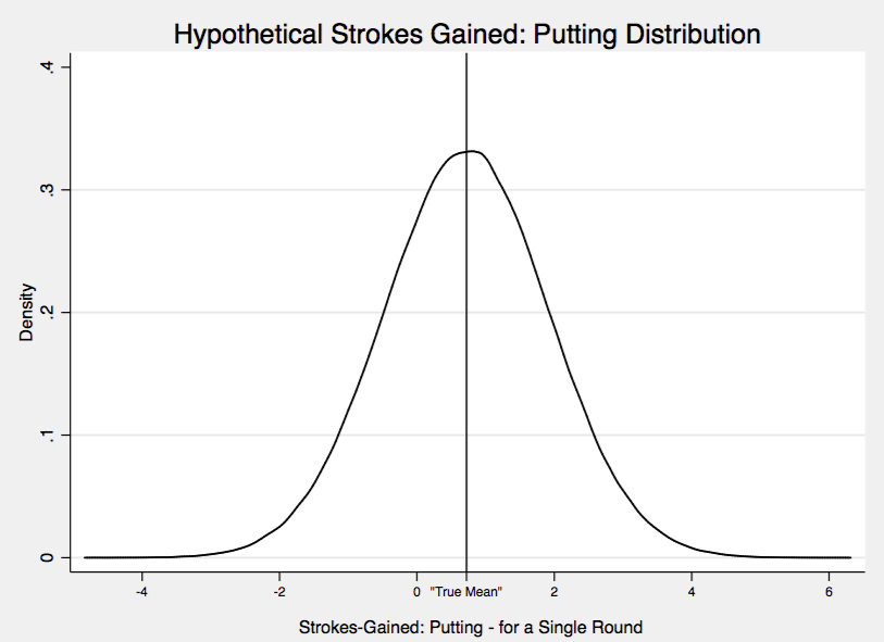
Loosely speaking, the y-axis indicates how likely an outcome is of occurring, and the x-axis specifies the range of values for SG:P. So the most likely outcome is the value labeled “True Mean”. We can imagine each player on the PGA Tour as having their own SG:P distribution. Better putters will have a “True Mean” shifted to the right, while worse putters will have it shifted to the left. If I could observe these distributions for a given year, I could easily rank the best putters by looking at their “True Means”. The problem is I do not observe these distributions, or these “True Means”. If, in a given year, I observed a huge number of SG:P for each player (thousands and thousands of rounds) I could trace out their respective distributions. However, I only observe about 50-80 rounds for each player in a year. The question is then, to what degree can I infer the “True Means” of players from a single year of data?
This is just a long-winded way of describing the basic problem of inferential statistics: I have a parameter (the “True Mean” above) that I could calculate exactly if I had an infinite amount of data, however I only observe a small sample (a year of PGA Tour data) from which I must draw my conclusions about this parameter.
Thus, we can think of the SG:P statistics reported by the PGA Tour as estimates of “True Means” for each player for that year. As estimates, they have a standard error associated with them. The standard error reflects the fact that if we had observed a different sample of rounds for a player we would have gotten a different estimate. Suppose I arbitrarily calculated the average SG:P for a player using the first half of the rounds he played in a year, and then did the same calculation using the second half of the year. I would almost surely obtain a different value for the average SG:P of that player with these two samples, even though these are both estimates of the same “True Mean” for that player. A standard error reflects the fact that the estimate varies with the sample used to calculate it.
The standard error is affected by two things; 1) the number of observations, and 2) the underlying variance of the SG:P distribution. The more observations, the smaller is the standard error. The smaller is the variance (i.e. the more horizontally compact the distribution I drew above is) the smaller is the standard error.
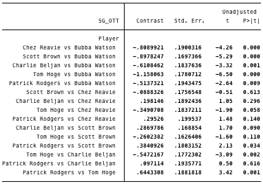
For the SG:P and SG:OTT statistics in 2015, I am going to analyze the 1st, 5th, 10th, 25th, 50th, and 100th players on the respective lists. I would like to conduct tests concerning the “True Means” of players occupying these different ranks. For example, Bubba Watson was 1st in SG:OTT, while Patrick Rodgers was 5th in SG:OTT; I would like to test whether the “True Mean” for Bubba was different from the “True Mean” of Rodgers in the year 2015. The following tables will summarize these tests.
In the tables below, “Contrast” gives the difference between SG:OTT (or SG:P) values, “Std. Err” is the standard error of this difference, and the informative number is the column titled “P>|t|”; this is called a p-value. It says the following: suppose that Bubba and Rodgers have the same “True Mean”, then the probability of observing the SG:OTT difference between Bubba and Rodgers at least as large as the one we did is equal to P>|t|. In the case of Bubba and Rodgers, there was only a 0.9% chance of observing a difference at least as large (in magnitude) as 0.514. The cutoff for what we call statistically significant is typically 5%. Anything below this, we say that we reject the null hypothesis that Bubba and Rodgers have the same “True Mean”. Thus, we have strong evidence that the difference between Bubba and Rodgers is due to Bubba having a higher “True Mean”, and not just sampling variability. Conversely, comparing Scott Brown (50th) and Chez Reavie (25th), we see that P>|t|=61%. This says that given Brown and Reavie have the same “True Mean” there is a 61% chance that we would observe the difference we did between their SG:OTT. This is very weak evidence that they have different “True Means”. Anyways, to the tables:
SG:OTT:
- 1st: Bubba Watson
- 5th: Patrick Rodgers
- 10th: Charlie Beljan
- 25th: Chez Reavie
- 50th: Scott Brown
- 100th: Tom Hoge
SG:P:
- 1st: Aaron Baddeley
- 5th: Brandt Snedeker
- 10th: Harris English
- 25th: Pat Perez
- 50th: Morgan Hoffmann
- 100th: Justin Rose
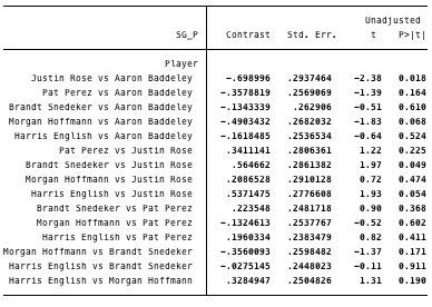
There are some very interesting results here. Notice that for the SG:P table, the only p-values that indicates statistical significance are the comparison of Rose (100th rank) and Baddeley (1st rank), and the comparison of Rose and Snedeker (5th rank). If we compare Hoffmann (50th) to Rose (100th) the p-value is 47% – not even close to statistical significance. This means that if Hoffmann and Rose have the same “True Mean”, there is still a 47% chance of observing a difference between their SG:P statistics as large as 0.21. One last example to make sure we understand – the p-value for Sneds (5th) and English (10th) is 91% – this means that it is very unlikely that their difference reflects differences in “True Means”. The take home message from the SG:P statistics is that the difference between a player ranked 50th and 100th is probably mostly just sampling noise – not ability. Similar thing with differences between 10th and 50th.
This is quite a contrast from our results for the SG:OTT statistic. If we compare Brown (50th) to Hoge (100th) the p-value is 11%. Not statistically significant, but much greater than the equivalent test with the SG:P statistic (47%). At this point, you should have the right idea on interpreting p-values, so look through the rest of the table. It is clear that SG:OTT rankings gives us much more information on “True Means” of players compared to the SG:P rankings.
To wrap things up, I’ve graphed the actual distributions for a few players in 2015 for SG:OTT and SG:P. This makes it clear why differences in SG:OTT are much more likely to reflect differences in actual ability, and not just statistical noise; the SG:OTT are much more concentrated around the mean (notice that the y-axis scales are equivalent on all graphs). A good driver of the ball like Bubba gains around 1.0 strokes per round a lot of the time. Conversely, Baddeley is a good putter but there is a much wider spread around his mean of 0.7. This makes perfect sense; you can’t fake a good driving round, while you can definitely fake a good putting round. Even terrible putters like Lee Westwood will have good putting days once in a while. However, a bad driver of the ball rarely will have days (read: never) where they drive it like Bubba does.
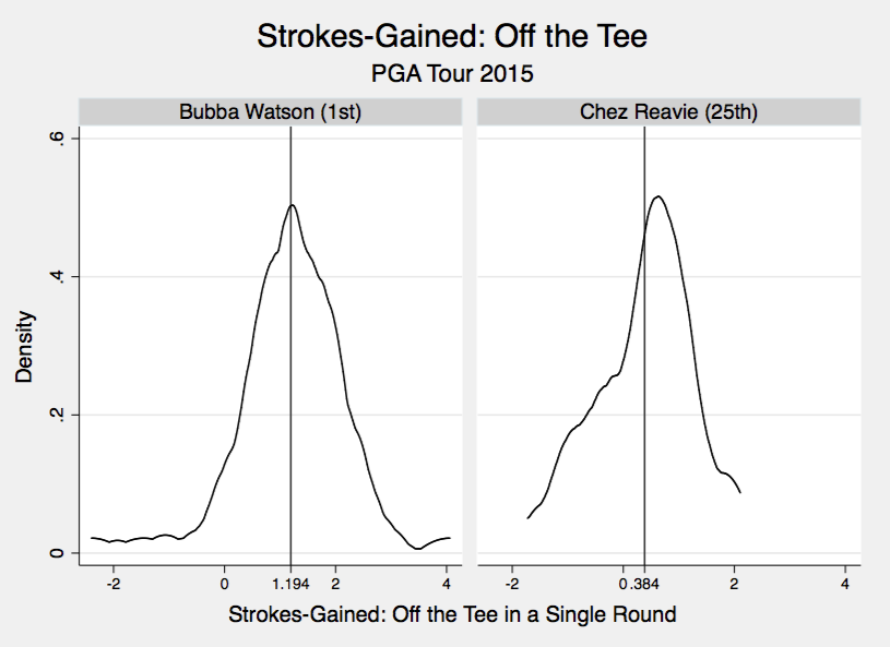
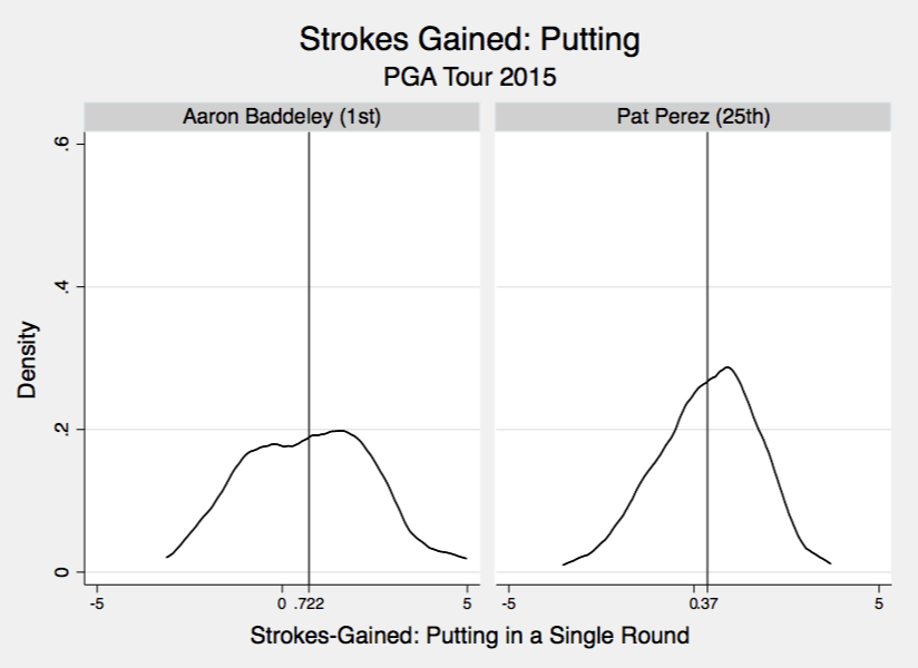
The take home message here is that annual SG:OTT values have a lot less statistical noise then the SG:P values do. Consequently, if you observe a player fall from 5th to 30th in SG:P from one year to the next I wouldn’t worry too much. However, if a player falls from 5th to 30th in SG:OTT, it is likely this actually reflects poorer driving ability that year.
All of this is not to say that the strokes-gained statistics don’t have value. They absolutely do, they are telling us where players are gaining strokes; that is a fact. The discussion here is about whether differences in SG statistics on a year-to-year basis reflect actual changes in player ability. Additionally, this analysis applies equally to any statistic collected by the PGA Tour. I wanted to focus on the strokes-gained stats as they are most important, it seems.
