The Hot-Hand Fallacy; Application to Golf

The existence of, and belief in,  a “hot-hand” in sports has long been a question of substantial interest to psychologists, economists, statisticians, and, of course, sports fans. The idea behind a “hot-hand” is that an individual is more likely to perform well following a good performance than they are following a poor performance. In basketball, which has been the context for most of the papers written on this subject, the question is whether a player is more likely to make a shot attempt given he made his previous shot attempt. In the ’80s and ’90s, a series of influential papers documented the absence of any hot-hand effect – in these studies players were no more likely (at least not to a statistically significant degree) to make a shot following a made attempt than they were following a missed attempt. These results got a lot of attention, and were largely rejected by the sports community who continued to believe in the hot-hand. This fueled more research documenting the irrationality of this belief and others like it; the common theme being that humans tend to give more meaning than they should to patterns in small samples of data.

However, there has been big news recently in this literature. The hot-hand fallacy result has been overturned in a paper by Joshua Miller and Adam Sanjurjo, which begins,

“Jack takes a coin from his pocket and decides to flip it, say, one hundred times. As he is curious about what outcome typically follows a heads, whenever he flips a heads he commits to writing the outcome of the next flip on the scrap of paper next to him. Upon completing the one hundred flips, Jack of course expects the proportion of heads written on the scrap of paper to be one-half. Shockingly, Jack is wrong. For a fair coin, the expected proportion of heads is smaller than one-half.”

As shocking as this statement is, it is true! You can check it by doing a simple simulation with some statistical software; I simulate a sequence of 50 coin flips, and calculate the proportion of heads that followed a head in the previous flip. I do this simulation 100,000 times and take the average of the proportions I get from each sequence, obtaining an average equal to 0.49! Crazy! As is explained at length in their paper, this is the result of a subtle selection bias. Honestly, it is hard to wrap your head around, and I won’t be able to provide an adequate explanation. Here is the link to their paper if you want to grapple with the concept for a bit. So, why is this relevant to understanding the hot-hand? Suppose a basketball player has a make percentage of 50%. Given what was described above, we know that in the absence of a hot-hand (i.e. the player shoots 50% regardless of whether he made or missed his previous shot(s)) the proportion of made shots following a made shot that we calculate from a sequence of data is expected to be strictly less than 0.5. Therefore, if we find in our data that the player made 50% of his shots following a made shot, this would actually be evidence in favor of this player having a hot-hand. This is due to the fact that our calculation of the proportion of made shots following a made shot is biased downwards.

In applying the concept of a hot-hand to golf, a relevant statistical summary could be the average score for a player conditional on the score they made on the previous hole (or previous two holes). You may wonder if the bias described above still persists when we are talking about non-binary (i.e. not 0 or 1, heads or tails, etc) outcomes. I answer this question with a brute force approach; I simulate 100 rolls of a die (i.e. I generate 100 numbers, each of which take on the values 1,2,3,4,5,6 with probability equal to 1/6), and then calculate the average value that followed a value of 1. I repeat this process 100,000 times and I find that the expected value of the die following a roll of 1 is about 3.53 (as opposed to 3.5, which is what it should be). By the same method, I find that the expected value of the die  following a roll of 2 is about 3.52, and so on, up to the expected value following a roll of 6 which is about 3.47. So it can be seen that the bias persists. Honestly, I still can’t believe that this is a thing; it truly is remarkable! I want to emphasize that, evidently, the expected value of a die after a 6 has been rolled is in fact 3.5 . But what these simulations show is that when we calculate this measure from data, in what would seem to be the most intuitive way to do so, our measure will be biased.

Back to golf; define outcomes in terms of relative score to par, so that a player’s relative score takes on integer values from -2 to 2 (ignoring any scores more extreme than this). A player who gets a hot-hand should have a lower expected score following a birdie than he would following a bogey. Formally, I define my measure of a player’s hot hand as the difference between their average score following a birdie, and their average score following a bogey. Thus, if this difference is negative that player performs better on holes that followed a birdie. Conversely, if the difference is positive that player performs better on holes that followed a bogey.

Given the discussion so far, if I take a sequence of hole scores, and calculate the average score on holes that follow a bogey, this average will be biased downwards. Conversely, the average score on holes following a birdie will be biased upwards. Therefore, just as in the case of basketball shooting data, my data will be biased to finding no evidence of a hot-hand.

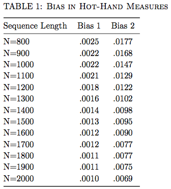
Importantly, this bias get smaller as the length of the sequence gets longer, but gets larger as you consider longer previous streaks (i.e. there is more bias when calculating the probability of a heads following 3 straight previous heads).

OK! Hopefully I still have some readers on board at this point, because I am heading to the data to figure out which golfers have a hot-hand.

Using 2016 PGA Tour ShotLink data, I calculate my hot-hand measure for each player as follows. I calculate the average score on holes that followed a birdie or better on the previous hole, and I calculate the average score on holes that followed a bogey or worse on the previous hole. I adjust the hole scores for hole difficulty by subtracting the average score on that hole that day. (This adjustment is made due to the concern that on easier courses players make more birdies, so, on average, the holes that follow their birdie holes are easier). The difference between these two averages will be my measure of that player’s hot-hand. However, I need to correct for the bias that will exist in each player’s measure. I don’t have an analytical expression for this bias, so I have to go the brute force route again; I simulate a sequence of scores (based on a typical score probability distribution; P(Eagle or Better)=1%; P(Birdie)=19%; P(Par)=63%; P(Bogey)=16%; P(Double or Worse)=2%). Then, I calculate the average of all values that follow a birdie or better in the sequence. Similarly, I calculate the average of all values that follow a bogey or worse in the sequence. I do this many times and calculate a grand average for each. Then, the difference between these two averages will be the bias present in my measure. This difference is equal to the bias because in my simulation there is no hot hand – it should be the case that the average score is independent of the previous hole’s score. Thus, if there was no bias in my simulations, the difference would be zero.

So, why would this bias be different for different players? Two things affect the bias; the probability distribution used to generate the data, and the length of the sequence. Because I am feeling lazy, I use the same probability distribution to generate simulated scores for every player (they are similar enough that it does not really matter in practice). Thus, the only difference between bias calculations for each player is the length of the sequence (i.e. the total number of holes that the player played in my sample).

Finally, I do all of which I just described again, except I consider how players perform following 2 consecutive birdies compared to following 2 consecutive bogies. As I mentioned earlier, this measure will carry a bigger bias with it. I refer to this measure as “Hot-Hand Measure 2”, while the previous measure is “Hot-Hand Measure 1”.

The following table shows the size of the bias in my two measures for sequences of various lengths that are relevant to the analysis.

The bias is much smaller for the measure that considers performance only on the previous hole. Additionally, both bias measures decrease as the sample length increases.

Next, some actual statistics.  The average hot-hand measures of all players on Tour in 2016 are shown below. This gives a sense of whether, on average, players tend to play better following good play on their previous hole(s).

 

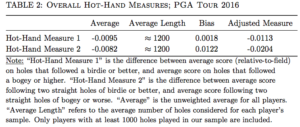
We see that, on average, PGA Tour players do experience the hot-hand phenomenon. Keep in mind that the first measure is much more precisely estimated than the second measure, due to the fact that there are more observations on players’ performance following a single birdie (bogey) then two consecutive birdies (bogies).

To get a sense of how meaningful the magnitudes of these measures are, note that -0.0113*18=0.20 and -0.0204*18=0.37. That is, if we imagine the average player playing an entire round in his “hot-hand state” (birdied previous hole) to his “cold-hand state” (bogied previous hole), this would result in a difference of 0.20 strokes (or 0.37 strokes in the case of our second measure). While this is certainly not a large difference, it is not nothing either. Additionally, as we will see next, there is a lot of individual heterogeneity in these hot-hand measures. Consequently, while this overall average is near zero, there are player-specific effects that are more meaningful in size.

The following interactive table provides the bias-corrected hot-hand measures for each player on the PGA Tour in 2016. The players at the top of these rankings could be considered the streakiest players, while the players at the bottom are anti-streaky; they play better, on average, following bogies than they do birdies. The overall ranking is determined by the sum of the rankings for Measure 1 and Measure 2.  You can sort based off either measure’s ranking by clicking on the column header.

For those interested, for hot-hand measure 1, there were typically 200-250 instances where a player made a birdie (bogey) in our sample. Therefore, our estimate for his average performance on the holes following a birdie (bogey) is based on 200-250 observations. This is a comfortably large sample size. For hot-hand measure 2, the average performance is based off a sample size of typically 40-50 observations. Consequently, you will notice there is much more variation in the hot-hand measure 2; this reflects the smaller sample size upon which the measure is constructed.

P.S. It has been pointed out to us that there have been papers written that are quite similar to this subject (or at least to the actual analysis we do). Here are the links Link 1 Link 2.