In this article we provide a method for comparing the performances of golfers who did not compete in the same time period. We answer questions of the following nature:
“How would the 2015 version of Rory McIlroy perform against the 1995 version of Greg Norman playing the same course with the same equipment?”
The statistical approach taken here is motivated by the method we use in our predictive model to adjust scores for field strength and course difficulty within a year (used in Broadie and Rendleman (2012), as well). In that context, because all European Tour and PGA Tour events contain overlapping sets of golfers, we are able to compare relative performances of all golfers even though all golfers do not directly compete against one another. The logic is that although Phil Mickelson and K.T. Kim may never play in the same tournament in a given year (suppose), because they both play in tournaments that contain Rory McIlroy, we are able to compare Mickelson and Kim through their performances relative to McIlroy.
The rest of this article is organized as follows: we first provide the intuition behind our approach, then provide results and a discussion of their interpretation, and then conclude with the statistical details.
Intuition
We use the same logic described above to compare players across generations. A macro example is shown here:
That is, we compare the performances of McIlroy and Faldo through their relative performances against Tiger. The method we use is based on this simple logic, but instead of just a single player linking players from different generations, we have hundreds. An obvious critique to this approach is that the Tiger Woods that Faldo played against was not necessarily the same Tiger Woods that McIlroy faced 10-15 years later. To get around this, we break each player’s career into 2-year blocks. So Tiger Woods in 1997-1998 is a “different player” in our sample than Tiger Woods in 1999-2000; his ability level can be different in the two periods. Therefore, to compare, for example, the 1995 version of Greg Norman to the 2015 version of Rory McIlroy, we first compare Norman to the players (that is, the 2-year blocks of players’ careers) he played against in 1995-1996, and then those players are compared to players they competed against in 1997-1998, and so on, all the way up to 2015.
Attentive readers may notice a problem here: the key to this approach is that we have overlap across time of players’ careers (i.e. part of Faldo’s career overlapped with Tiger, and part of Tiger’s overlapped with Rory), but now that we have defined each 2-year segment of a player’s career as distinct, how do we ensure we still have overlap? That is, if every player from 1999-2000 is a distinct “player” from that in 2001-2002, then we have no way to link the performances of these two groups of players. We circumvent this problem by randomly assigning half the players in our sample to have their 2-year blocks defined starting on the odd years (1999-2000, 2001-2002), and the other half of the sample starts on the even years (2000-2001, 2002-2003). Therefore, we are able to link the performance of say, the 2000-2001 version of Tiger to the 2002-2003 version of Tiger by comparing his performances to 2001-2002 Mickelson (because both 2000-2001 version of Tiger and 2002-2003 version of Tiger competed against the 2001-2002 version of Mickelson). For our results, we actually end up getting a value for a player’s performance in each year of their career (this is discussed in detail later). This annual measure should be thought of as a sort of smoothed 3-year average (i.e. Tiger’s 2000 value is affected by his 1999 and 2001 performances as well).
The main assumption we are relying on is that within a 2-year period players’ ability is constant on average. There can be some players whose performance improves during a 2-year period as long as there are others whose performance declines. We require that on average these discrepancies even out.
In Connolly and Rendleman (2008), they estimate a continuous time-varying golfer-specific ability function. However, for our purposes, we cannot implement this; there would be no way to separate genuine changes in player ability over time from technological advances or improvements in course conditions.
Ranking PGA Tour Players from 1984-2016
We are using PGA Tour round-level data from 1983-2017 (the reason we have to drop the first and last years in the sample is explained in a later section). The output of this method is a value for each year of each player’s career in our sample. This value is going to be measure of that player’s performance in that year; we call this the All-Time Performance Index (ATPI).
The ATPI is a relative measure, and as such it requires a normalization. The absolute level of the index is irrelevant, what matters is the relative magnitudes. We decide to give the average player on the PGA Tour in the year 2000 an ATPI of zero. The interpretation of the index is best understood with a specific example. The ATPI value of 3.8 assigned to Rory McIlroy in 2015 says the following: the 2015 version of McIlroy would be expected to beat the average PGA Tour player in the year 2000 by 3.8 strokes in a single round, on the same course using the same equipment. Therefore, the ATPI value for each player-year observation represents their scoring average on a “neutral” course relative to the average player in the year 2000.
Okay, now to some results (which some people are not going to like, or believe, perhaps). As usual, the plots are interactive so click around.
First, we plot the average ATPI across all players (weighted by the number of rounds played) for each year from 1984-2016. Additionally, we plot the ATPI for the best player in each year.
The aggregate annual numbers reflect the expected scoring difference in a single round between the average player in the relevant year and the average player in the year 2000.
Next, we basically provide all the ATPI data in this interactive graph. From the dropdown bar choose any player, and his ATPI for all years in which he played a minimum of 25 rounds will be plotted.
If you are doubting the validity of the results, please take a long look through the data. Looking at individual players' ATPI over the span of their careers has helped convince us of the validity of this measure. For example, if you think that our measure is systematically biased to favor more recent players, then we should (in general) observe players' ATPI steadily rising over their careers (even if their true ability stays relatively constant). Look up some players that have their entire career contained within 1984-2016 (Leonard, Vijay, Love III, for example). If the measure is not biased to recent years, you should observe a career arc in a player's ATPI, where they peak in the middle of their career, and have lower quality performance at the beginning and end of their careers. This is generally what you find.
Next, here are the best player-years of all-time according to the ATPI:
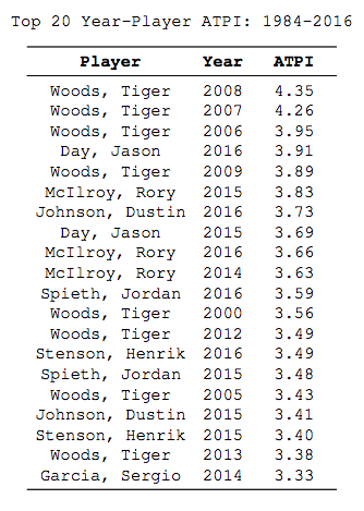
This highlights Tiger's greatness, as well as the strength of today's best players.
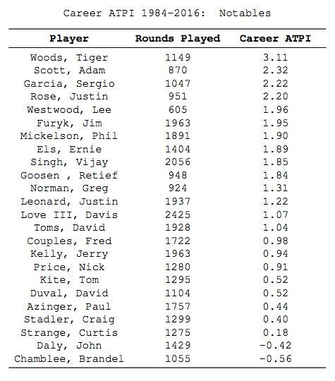
Finally, we provide a list of some notable players' average ATPI over the entire sample period. The players listed are generally those who have all (or most) of their careers contained in our 1984-2016 sample. Keep in mind that, for most of these players, (relatively) poor performances in the last few years of their careers causes their careers ATPI averages to be a bit lower than in their primes.
So... What to Make of This?
If you are willing to accept the assumptions imposed by this approach, the interpretation of these numbers is as has been stated above. That is, the differences between players' ATPI reflect differences in single-round scoring average in a neutral setting (i.e. technology, course conditions, etc are held constant). If you are uncertain as to whether we are controlling for technology changes or course conditions, recall the simple example given earlier: Rory is compared to Tiger (they are using the same equipment and playing the same courses), and Tiger is then compared to Faldo (they are also using the same equipment and playing the same courses). And, through this, Rory and Faldo are compared.
Of course, we don't think this analysis proves that mid-level players today should be regarded as "greater" golfers than Greg Norman or Tom Watson, for example. The greatness of any athlete will always be measured by their performances relative to their peers. In athletics, Roger Bannister was the first man to break the 4-minute mile barrier, and is held in very high regard because of it - despite the fact that the best high school boys can break 4 minutes in the mile today (although some of that would be attributed to improvements in shoes and track surfaces).
It very well could be that if Greg Norman had grown up in the same generation as McIlroy, he would be better than McIlroy. This analysis cannot speak to the validity of that claim. The current generation has modern technology and improved coaching (whether the latter is helpful could be debated) at their disposal to aid the development of their games in their formative years. Further, serious fitness routines have become the norm among competitive golfers. Finally, and we think most importantly, the raw numbers of serious golfers has grown immensely in the last 30 years, resulting in an increased level of competition that pushes all golfers to get better.
All of these factors could contribute to better performances by recent generations of golfers. It seems natural to think that all sports are continually progressing, and current athletes always have a bit of an edge over those that preceded them.
Statistical Details
Our results are based on fixed-effects regressions of the following form:
\( Score_{ijt} = \mu_{i,t;t+/-1} + \delta_{jt} + \epsilon_{ijt} \)
where i is indexing player, j is indexing a specific tournament-round, and t is indexing time. The slightly complex subscript i,t;t+/-1 is indexing a specific player in the years t and t+1, or t and t-1 (depending whether the player has 2-year blocks on odd or even years).
In practice, this is implemented as a regression of score on a set of dummy variables for each 2-year block of a player's career and a set of year-tournament-round dummies.
As described earlier, we need overlap between the 2-year segments of different players' careers to connect performances across time. To obtain this overlap, we randomly assign half the players in our sample to have 2-year blocks starting on the even years (2010-2011, 2012-2013), while the other half gets the odd years (2011-2012, 2013-2014). Evidently, we do not want our estimation procedure to be sensitive to this assignment; therefore, we run the estimation many times. Because assignment is random, in some years a player will be assigned to odd-numbered 2-year segments, while in others they will be assigned to even-numbered 2-year segments. In each estimation iteration we collect the player fixed effects for every year of their career (they will be the same for each 2-year block), and then the ATPI will be calculated as the average value for a given year over all estimation iterations.
Let's make this concrete with an example; I'll describe how we come up with Rory McIlroy's ATPI for 2015. Suppose in the first estimation iteration Rory is assigned to be on the even years for his 2-year blocks. We run the regression, and obtain Rory's fixed effect for 2014-2015 (suppose it is 4.0). We write down this value as a measure of Rory's performance in the years 2014 and 2015. Next, suppose on the second iteration Rory is assigned to be on the odd 2-year block. Now, we run the regression and obtain Rory's fixed effect for 2015-2016 (suppose it's 3.0). We write down this value as a measure of Rory's performance in the years 2015 and 2016. If we decided just to do 2 iterations, Rory's ATPI value for 2015 would be equal to (3.0 + 4.0) / 2 = 3.5. Therefore, it is best to think of Rory's 2015 ATPI as a type of smoothed 3-year average, as it is ultimately obtained by averaging estimates of his performance for the 2-year blocks 2014-2015 and 2015-2016 (clearly, the middle year influences this average the most).
The fixed effects estimation is fairly computationally difficult, so we perform just 100 iterations. The estimates do not vary drastically from one iteration to the next, and consequently we think 100 iterations is more than enough to get rid of any statistical oddities that could appear from the random assignment. We drop the first and last years, 1983 and 2017, as the estimation procedure requires that there is a year on either side of the year of interest.
To conclude, it is worth mentioning the work in Berry, Reese, and Larkey (1999), who used a conceptually similar method to compare the performances of players in major championships over 5 decades. Their results are also very interesting.